1. Stereo Matching

1.1. Camera Model

Camera model is required in calculating the 3D points from the disparity image. Camera parameters are of two sorts, (a) intrinsic camera parameters and (b) extrinsic camera parameters. Intrinsic corresponds to the focal lengths and principal axis points, while extrinsic parameters are the camera rotation and translation with respect to a known word point.

The functionality of a camera is that it projects a 3D world point into a 2D image plane. This transformation is approximated using the projection matrix, which is also known as the camera matrix. Camera matrix is a combination from intrinsic matrix and extrinsic matrix. Extrinsic matrix is a combination of rotation and translation matrices, used for conversion from the world model to camera model. Camera matrix is derived based on the pin-hole camera model, which is presented below.

(1.4)\[\begin{split}\begin{equation} \begin{bmatrix} \tilde{x} \\ \tilde{y} \\ \tilde{w} \end{bmatrix}= {K}_{3 \times 3} \begin{bmatrix} R_{3 \times 3} & T_{3 \times 1} \end{bmatrix} \begin{bmatrix} X \\ Y \\ Z \\ 1 \end{bmatrix} \end{equation}\end{split}\]

(1.5)\[\begin{split}\begin{equation} K= \begin{bmatrix} f_x & 0 & c_x \\ 0 & f_y & c_y \\ 0 & 0 & 1 \end{bmatrix} \end{equation}\end{split}\]

(1.6)\[\begin{equation} u=\dfrac{\tilde{x}}{\tilde{w}} \hspace{1cm} v=\dfrac{\tilde{y}}{\tilde{w}} \end{equation}\]

(1.7)\[\begin{equation} f_x=\dfrac{F}{p_x} \hspace{1cm} f_y=\dfrac{F}{p_y} \end{equation}\]

In above (1.4), (1.5), (1.6) and (1.7) , \((u,v)\) are the image co-ordinates in pixel units while \((X,Y,Z)\) is corresponding world point in world measurement units. \(F\) and \((p_x,p_y)\) are focal length and pixel dimensions (height and width) expressed in world units and \((f_x,f_y)\) are focal length in pixel units. These equations show how a 3D world co-ordinate is transformed to a 2D image plane. In (1.4) above, \(K\) denotes the intrinsic camera matrix while \(R\) and \(T\) are rotation and translation matrices which together forms the extrinsic camera matrix. Intrinsic camera matrix is independent of the scene and hence can be reused as long as the camera focal length remains unchanged. On the other hand extrinsic matrix translate 3D world co-ordinate to camera co-ordinate system. Point in the world co-ordinate system \((X,Y,Z)\) and same point in camera co-ordinate system as \((x,y,z)\), can be expressed as in (1.8).

(1.8)\[\begin{split}\begin{equation} \begin{bmatrix} x \\ y \\ z \end{bmatrix} = R \begin{bmatrix} X \\ Y \\ Z \\ 1 \end{bmatrix} + T \end{equation}\end{split}\]

Hence we can derive image points \((u,v)\), simply in the below manner.

(1.9)\[\begin{equation} u = f_x \times \acute{x} + c_x \hspace{1cm} v = f_y \times \acute{y} + c_y \end{equation}\]

where;

(1.10)\[\begin{equation} \label{eq:ch2-13} \acute{x} = x/z \hspace{1cm} \acute{y} = y/z \end{equation}\]

Camera distortion is common phenomenon which occurs to imperfect manufacturing and properties associated with lenses. Distortion parameters are also of two sorts, which are (a) radial distortion and (b) tangential distortion. Radial distortion occurs because the light rays bend more near the edge of the lens compared to the lens optical center. Tangential distortion occurs when the lens and the image plane are not parallel to each other. The above mentioned camera model is for a pin-hole camera and needs to be adjusted for the distortion parameters. So the model is extended as below. \(T_D\) represent tangential distortion while \(R_D\) represent radial distortion.

(1.11)\[\begin{equation} u=f_x \bigg( x'\frac{1+D_{r1}r^2+D_{r2}r^4+D_{r3}r^6}{1+D_{r4}r^2+D_{r5}r^4+D_{r6}r^6} + 2D_{t1}x'y'+D_{t2}(r^2+2x'^2) \bigg)+c_x \end{equation}\]

(1.12)\[\begin{equation} v=f_y \bigg( y'\frac{1+D_{r1}r^2+D_{r2}r^4+D_{r3}r^6}{1+D_{r4}r^2+D_{r5}r^4+D_{r6}r^6} + D_{t1}(r^2+2y'^2)+2D_{t2}x'y' \bigg)+c_y \end{equation}\]

where;

(1.13)\[\begin{equation} r^2 = x'^2 + y'^2 \end{equation}\]

(1.14)\[\begin{equation} R_D = (D_{r1} , D_{r2} , D_{r3} , D_{r4} , D_{r5}, D_{r6}) \end{equation}\]

(1.15)\[\begin{equation} T_D = (D_{t1} , D_{t2}) \end{equation}\]

Aim of camera calibration is to find the parameters to model the above mentioned camera model. There are off-the shelf implementations in both Matlab and OpenCV for camera calibration. Even though there are six parameters used to model radial distortion, three parameters are sufficient to model the current lens distortions. Distortion is dominated by radial distortion components. Calibrating a stereo camera pair requires an additional step, which is to calculate the rotation and translation of the second camera (usually the right camera) with respect to the first camera (usually the left camera). These calibration parameters (intrinsic and extrinsic parameters, radial and tangential distortion parameters) are required to perform rectified images when solving the correspondence problem efficiently and estimating the 3D world coordinates for disparity values.

1.2. 3D Estimation

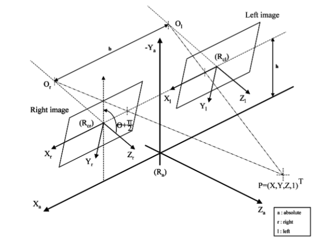
Fig. 1.2 Stereo system and co-ordinate system

Using the equations described in (1.4), (1.5), (1.6), the mapping between the world co-ordinates \((X,Y,Z)\) and the image co-ordinates \((u,v)\) can be found. According to the above Fig. 1.2, (1.4) can be defined as below (1.16).

(1.16)\[\begin{split}\begin{equation} \begin{bmatrix} \tilde{x} \\ \tilde{y} \\ \tilde{w} \end{bmatrix}= \begin{bmatrix} f_x & 0 & c_x \\ 0 & f_y & c_y \\ 0 & 0 & 1 \end{bmatrix} \begin{bmatrix} 1 & 0 & 0 & -\varepsilon_i\dfrac{b}{2}\\ 0 & cos\theta & -sin\theta & h\\ 0 & sin\theta & cos\theta & 0 \end{bmatrix} \begin{bmatrix} X \\ Y \\ Z \\ 1 \end{bmatrix} \end{equation}\end{split}\]

where \(\theta\) is the angle between the optical axis of the cameras \(O_rR_{cr}, O_lR_{cl}\) and the horizontal axis. \(b\) is the baseline, which is the distance between the camera optical centres and \(h\) is the height of the cameras mounted from the origin. \(\varepsilon_i\) is a constant where \(\varepsilon_i=-1\) for left image and \(\varepsilon_i=1\) for the right image.

The roll angle \(\theta\) can be made negligible when mounting the cameras in the vehicle by making the camera rig parallel to the road surface. This simple trick will reduce the complexity of (1.16) as \(\theta\approx0\) will make \(sin\theta\approx0\) and \(cos\theta\approx1\). Furthermore, if the origin is assumed to be at the optical center of the left image, (1.16) can be re-written as below (1.17) for the left image and (1.18) for the right image.

(1.17)\[\begin{split}\begin{equation} \begin{bmatrix} \tilde{x} \\ \tilde{y} \\ \tilde{w} \end{bmatrix}= \begin{bmatrix} f_x & 0 & c_x \\ 0 & f_y & c_y \\ 0 & 0 & 1 \end{bmatrix} \begin{bmatrix} 1 & 0 & 0 & 0\\ 0 & 1 & 0 & 0\\ 0 & 0 & 1 & 0 \end{bmatrix} \begin{bmatrix} X \\ Y \\ Z \\ 1 \end{bmatrix} \end{equation}\end{split}\]

(1.18)\[\begin{split}\begin{equation} \begin{bmatrix} \tilde{x} \\ \tilde{y} \\ \tilde{w} \end{bmatrix}= \begin{bmatrix} f_x & 0 & c_x \\ 0 & f_y & c_y \\ 0 & 0 & 1 \end{bmatrix} \begin{bmatrix} 1 & 0 & 0 & -b\\ 0 & 1 & 0 & 0\\ 0 & 0 & 1 & 0 \end{bmatrix} \begin{bmatrix} X \\ Y \\ Z \\ 1 \end{bmatrix} \end{equation}\end{split}\]

If the left image is considered, i.e.:eq:eq:ch2-20 the relationships between the physical world and image world can be derived using (1.19) and (1.20).

(1.19)\[\begin{equation} u=\dfrac{\tilde{x}}{\tilde{w}}=c_x+\dfrac{f_xX}{Z} \end{equation}\]

(1.20)\[\begin{equation} v=\dfrac{\tilde{y}}{\tilde{w}}=c_y+\dfrac{f_yY}{Z} \end{equation}\]

Now there are two equations to find the three world co-ordinates \((X,Y,Z)\). Given an image point, the image co-ordinate \((u,v)\) and with calibration \(c_x, c_x, f_x\) and \(f_y\) are known. Consider \(PO_rO_l'\) triangle in the Fig. 1.3 which represent a rectified stereo camera system with parallel epipolar lines, to arrive at (1.21).

(1.21)\[\begin{equation} Z=f\dfrac{b}{u_l-u_r}=f\dfrac{b}{d} \end{equation}\]

where \(f\) is the focal length of the camera system. General assumption in such stereo systems is that \(f\approx f_x\approx f_y\), where we can easily find the \(f\) by taking the average of the \(f_x\) and \(f_y\) of the two cameras. The baseline \(b\) can be found from the calibration process. This process of determining depth from disparity \(d\) is known as \(triangulation\). Note that depth \(Z\) is inversely proportional to disparity \(d\).

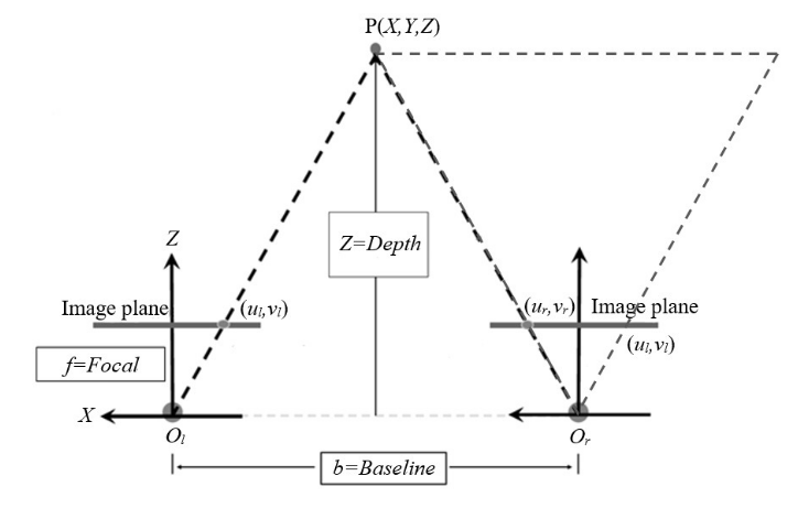
Fig. 1.3 Stereo system with parallel epipolar lines

Therefore, with this configuration the depth \(Z\) for all the pixels \((u,v)\) in the left image for which disparity value \(d\) is known can be calculated using (1.21). Then by using (1.19) and (1.20), \(X\) and \(Y\) co-ordinates can be found, which will give the 3D world co-ordinate. However, a dense disparity map will only provide a sparse 3D map as a pixel-level disparity value will not provide a continuous depth field but only step-wise depth values.

1.3. Image Rectification

Two main challengers in correspondence problem are (a) how to match and (b) what to match. The first can be simply done by conducting a 2D search in one image to a reference point in the other. However, this is a very time consuming process which can be efficiently solve using rectification. With image rectification 2D search can be minimized to a 1D search using the principles of Epipolar Geometry.

Fig. 1.4 Epipolar Geometry

In the Fig. 1.4, \(O_l\) and \(O_r\) are the two camera centers and \(O_lO_r\) is the 3D line connecting the two camera centers which intersects the left and right image planes at \(E_l\) and \(E_r\), which are called epipolar points.:math:O_lPO_r plane is termed as the epipolar plane. All the points in the world line \(O_lP\) is seen by the right camera image plane \(p_rE_r\) line. Therefore when you need to search for a match for point \(P\) in the world which is also a point in \(O_lP\) line, you only need to search in the corresponding epipolar line \(p_rE_r\) in the right image. This is effectively reducing your 2D search into a 1D search. Given a point \(p(u,v)\) in an image corresponding epipolar line \(l'\) in the other image can easily be found using (1.22) mentioned below, where \(F\) is the Fundamental Matrix between two images. Fundamental matrix can be easily found using intrinsic and extrinsic parameters, which is common knowledge in stereo vision.

(1.22)\[\begin{equation} l' = F.p(u,v) \end{equation}\]

With help of epipolar geometry, 2D search has been reduced to a 1D search. However scanning an arbitrary line is also inefficient in image processing. In order to address this epipolar lines are made horizontal and parallel to each other. This is when epipolar points are placed at infinity. This process is known as stereo image rectification. Once you have rectified image pair, match to a point in one image can be found just scanning a horizontal line in the other. Refer to the Fig. 1.5 below to visualize the results.

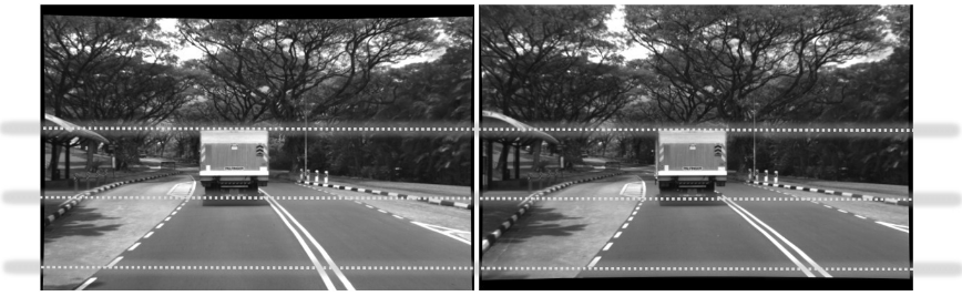
Fig. 1.5 Rectified images

1.4. Stereo Matching using SGM

Stereo matching is the process of finding the corresponding points between the let and right images and calculating the disparity for each pixel on the image based on that. Generating matching points between the two frames is known as the correspondence problem. Once matching correspondences are generated disparity value is the co-ordinates (pixel positions in the two image views) difference between the two pixels corresponding to the same point in the world. Fig. 1.6 visualize this situation and mathematical representation for disparity \(d\) calculation is given in (1.23) where subscript \(l\) and \(r\) are to indicate left and right image views.

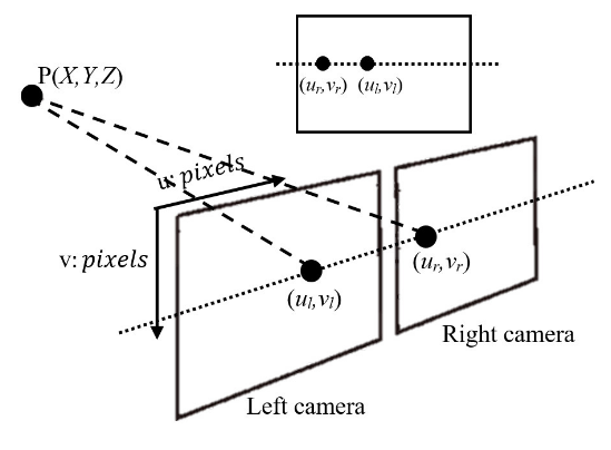
Fig. 1.6 Disparity from stereo vision

(1.23)\[\begin{equation} \label{eq:ch2-1} d = u_l - u_r \end{equation}\]

Once the images have been rectified the other problem to be addressed is how to define a good metric to match the points between two images. there are two main types of stereo matching algorithms in traditional stereo matching approaches, which are (a) local stereo methods and (b) global stereo methods. Main difference in these two methods are based on how each algorithm performs optimization, whether the optimization is done locally or globally. Moreover, stereo matching process is divided into four parts, namely (1) matching cost computation, (2) cost aggregation, (3) disparity calculation and optimization and (4) disparity refinement.

We make use of the GPU based stereo matching code publicly made available called libSGM. This follows the Semi Global Matching (SGM) stereo matching method proposed by Hirschmüller, Heiko in “Accurate and efficient stereo processing by semi-global matching and mutual information.”, where for the per-pixel matching cost calculation instead of Mutual Information, Census transformation is used. We will breifly describe the process for better understanding.

The matching cost calculation is done using Mutual Information which is defined based on the entropy (on intensity information) of the two images and joined entropy. Entropy is calculated from the probability distributions of the intensity values on the two images. Instead of using the whole image, they have used information of a neighbourhood window. However in the implementation, matching cost is calculated based on Census Transformation. Census Transformation is generated based on the intensity values of pixels inside a window. If you consider \(3\times3\) window Census Transform is a eight bit codeword, where the intensity value of the center pixel is compared with the eight pixels in the \(3\times3\) neighbourhood in arriving at the eight bit code word. This can be arrived from clockwise direction or anti-clockwise direction, but should adhere to one direction throughout the implementation. If the center pixel intensity is higher than that of the neighbouring pixel in consideration, bit is set to 1 and 0 otherwise. Same convention is followed through out. Different matching cost methods have been analysed for best performance in both local and global optimization methods. Based on the results authors state that Census Transformation based matching cost has yeilded better results than other methods (this analysis also includes Mutual Information), except when the image is corrupted with strong noise. Therefore using Census Trasformation over Mutual Information can be validated. Hamming distance as used for the per pixel cost for a 16 bit codeword generated considering 16 selected pixels from \(9\times9\) window. Hamming distance is a measurement of the minimum number of bit changes required to match two codewords.

Cost aggregation and optimization is done based on multi directional Dynamic Programming approach. First an energy function is defined, which is as per (1.24).

(1.24)\[\begin{equation} E(d) = \sum_{p}C(p,d_p) + \sum_{q \in N_p}P_1T[\mid d_p-d_q \mid=1] + \sum_{q \in N_p}P_2T[\mid d_p-d_q \mid>1] \end{equation}\]

where \(d\) stands for disparity and \(q\) are pixels in the \(p\) neighbourhood \(N_p\). \(P_1\) and \(P_2\) are penalty terms and \(C(p,d_p)\) is the data term coming from the matching cost. Other two terms are smoothness terms where in the neighbourhood if there is one pixel difference in disparity small panelty \(P_1\) is added and for higher disparity difference larger panelty \(P_2\) is added. This method supports adaptation to slanted surfaces with smaller panelty and preserves discountinuities with a constant panelty for larger differences. Optimizing \(E(d)\) is a time consuming process. Hence, authors propose multi directional 1D Dynamic Programming approach in doing it efficiently. This can be explained based on (1.25).

(1.25)\[\begin{split}\begin{align} L_r(p,d) & = C(p,d) + min \{ L_r(p-r,d), L_r(p-r,d-1) \\ & +P_1, L_r(p-r,d+1)+P_1, min_iL_r(p-r,i)+P_2 \}- min_kL_r(p-r,k) \end{align}\end{split}\]

where \(L_r\) is the 1D path travelled in the \(r\) direction and \(C(p,d)\) pixel matching cost. So the pixel matching cost is added with the lowest cost of the previous pixel \(p-r\) of the path with panelties for smoothness enforcements and then minimum path cost (for any disparity) deducted from that. The third term is to refrain \(L_r\) continuing to increase along the path. This can be seen as a 1D implementation of (1.26). To arrive at the aggregated cost \(L_r\) from all \(r\) are summed as in (1.26).

(1.26)\[\begin{equation} S(p,d) = \sum_{r}L_r(p,d) \end{equation}\]

Authors suggest that at least eight directions should be considered for good results. However, we have seen good results even at four directions, which will reduce the running time considerably. Disparity value is then selected using a Winner Takes All approach from \((p,d)\) that corresponds to the minimum cost (\(min_dS(p,d)\)). Hence the name Semi Global Matching (SGM) method. Once the disparity map is generated for the base image, disparity map is generated for the matched image using the same path costs calculated and following a WTA approach. If the disparity values for the same point differ more than one pixel its disparity value is marked as invalid. Hence a dense disparity map is generated with possible missing values due to invalidation.

Stereo matching method is implemented using CUDA for GPU support to make the algorithm achieve real time performance. We use a disparity search range upto maximum of 128 pixels in our implementations. In order to further improve the calculation time we use half sized images from the originally captured images. With this configuration, detect points at 5 m to 45 m even though the system is capable of distances up to 57 m.